Moldex3D for Conformal Cooling Simulation: Setup, Workflow & Accuracy

1. What Moldex3D Brings to Conformal Cooling Analysis

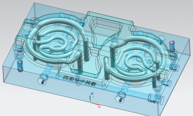
Moldex3D is a true 3D CAE simulation platform for injection molding that uses a proprietary BLM (Boundary Layer Mesh) solver. Unlike solvers that approximate cooling channels as 1D beam elements, Moldex3D meshes the entire mold block, cooling channels, and part cavity as interconnected 3D solid elements. This distinction becomes critical when you move from straight-drilled cooling lines to conformal cooling channels, where the channel cross-section may be oval, teardrop-shaped, or D-shaped, and the channel path follows the contour of the part surface at variable wall-to-channel distances.

For conformal cooling simulation, the 3D solid approach captures three phenomena that beam-element solvers miss:

• Non-uniform heat transfer coefficients around non-circular channel cross-sections, where the inner and outer radii of a curved channel see different flow velocities and therefore different convective heat transfer rates.
• Conduction bridging between closely spaced conformal channels, where the thermal interaction between adjacent channels affects the overall mold temperature field.
• Insert-to-base thermal contact resistance at the interface between a 3D-printed conformal insert (typically maraging steel or MS1) and the conventionally machined mold base (typically P20 or H13).

These capabilities make Moldex3D a strong choice for engineers who need to validate conformal cooling channel designs before committing to expensive metal 3D printing. The software is developed by CoreTech System in Taiwan and is widely used across Asia, Europe, and North America.

2. Setting Up a Conformal Cooling Simulation in Moldex3D

The setup process in Moldex3D differs from conventional cooling analysis primarily in meshing. Conformal channels demand more mesh refinement because of their complex geometry. Here is the step-by-step workflow:

3. Key Simulation Outputs and What They Mean

After the simulation completes, Moldex3D produces several output fields that are critical for evaluating conformal cooling design effectiveness:

Cooling Time

The time required for the hottest point in the part to reach ejection temperature. For conformal cooling, expect 20–40% reduction compared to conventional straight-drilled channels. If Moldex3D shows less than 10% improvement, the channel layout likely has coverage gaps or the channels are too far from the cavity surface.

Mold Surface Temperature Distribution

This is the most important output for conformal cooling evaluation. Look at the temperature range (delta T) across the cavity surface at end of cooling. A well-designed conformal circuit should achieve a delta T of less than 5 degrees C across the entire cavity surface. Conventional cooling typically shows 15–30 degrees C variation. Temperature uniformity directly correlates with warpage reduction and surface quality improvement.

Warpage Prediction

Moldex3D predicts total warpage as a displacement field on the part. For conformal cooling validation, compare the warpage magnitude and pattern between the conventional cooling baseline and the conformal design. Typical warpage reduction is 30–60%. The warpage analysis uses the temperature field from the cooling analysis as input, so errors in the cooling prediction propagate directly into the warpage result.

Coolant Pressure Drop

The pressure drop through the conformal circuit determines whether the channels can be adequately fed by the mold temperature controller (MTC). Moldex3D calculates pressure drop based on the actual 3D channel geometry. For conformal channels, pressure drop is typically 1.5–3x higher than conventional straight channels due to the curved paths. If the predicted pressure drop exceeds 3 bar, consider increasing the channel diameter or splitting the circuit into parallel branches.

Volumetric Shrinkage

Uniform cooling from conformal channels reduces the variation in volumetric shrinkage across the part, which is the root cause of warpage. Look at the shrinkage contour plot for hot spots — areas of high shrinkage indicate insufficient cooling coverage.

4. Moldex3D vs. Moldflow for Conformal Cooling Analysis

Both Moldex3D and Autodesk Moldflow can simulate conformal cooling, but they use fundamentally different approaches to channel modeling. Here is a detailed comparison:

Feature	Moldex3D (BLM Solver)	Moldflow (Beam Element)
Channel mesh type	3D solid with boundary layers	1D beam elements
Non-circular cross-sections	Fully resolved geometry	Approximated as equivalent circular
Channel-to-channel thermal interaction	Captured via 3D conduction	Not directly modeled
Insert/base contact resistance	Definable interface condition	Requires manual workaround
Transient cyclic analysis	Built-in, up to N cycles	Built-in, up to N cycles
Warpage prediction accuracy	High (3D thermal input)	Moderate (interpolated thermal input)
Solver speed (single cavity)	30–60 min (high element count)	10–25 min (lower element count)
Learning curve	Steeper (manual mesh control)	Gentler (more automated)
DOE / optimization	Built-in DOE module	Built-in DOE module
Licensing cost (annual)	$15,000–$45,000	$18,000–$50,000

For conventional straight-drilled cooling, both platforms give comparable results. The accuracy gap widens when channels deviate from circular cross-sections and follow complex 3D paths — this is where Moldex3D's solid mesh approach provides measurably better temperature and warpage predictions.

5. Moldex3D Designer BLM vs. eDesign Workflow

Moldex3D offers two primary workflows for conformal cooling simulation. Choosing the right one depends on your project stage and accuracy requirements.

Aspect	Designer BLM (Desktop)	eDesign (Cloud)
Mesh control	Full manual control over element size, boundary layers, local refinement	Automated meshing with limited user control
Channel geometry handling	Imports full 3D solid channel geometry	Supports channels but simplifies complex geometry
Solver options	Transient, steady-state, coupled, DOE	Standard analysis types
Post-processing	Full 3D visualization, cross-section probes, export to CSV	Web-based viewer with basic probes
Best use case	Final validation of conformal design	Feasibility screening, concept comparison
Hardware requirement	Workstation with 32+ GB RAM	Web browser only
Typical solve time	30–90 min (local compute)	15–45 min (cloud compute)

6. Interpreting Results: Temperature Bands and Pressure Drop Thresholds

What Delta-T Bands Mean

The temperature variation (delta T) across the mold cavity surface at the end of cooling is the single most important metric for evaluating conformal cooling performance. Here is how to interpret the numbers:

Delta T Range	Rating	Interpretation
< 3 °C	Excellent	Minimal warpage risk. Suitable for tight-tolerance parts, optical components, and class-A surfaces.
3–5 °C	Good	Acceptable for most injection molding applications. Standard target for conformal cooling designs.
5–10 °C	Marginal	Some warpage risk on thin-wall parts. May be acceptable for structural parts without cosmetic requirements.
10–15 °C	Poor	Likely warpage issues. Conformal design needs revision — check for coverage gaps or channels too far from cavity.
> 15 °C	Unacceptable	No significant improvement over conventional cooling. Redesign the channel layout.

Pressure Drop Thresholds

Coolant pressure drop through the conformal circuit must be compatible with the mold temperature controller's pump capacity. Exceeding the MTC's pressure capability results in reduced flow rate, turbulence loss, and degraded cooling performance.

A common design mistake is to make conformal channels too small (under 4 mm diameter) in pursuit of maximum cooling surface area. While smaller channels allow placement closer to the cavity, the pressure drop increases with the fourth power of the diameter reduction. A 4 mm channel has 5x the pressure drop of a 6 mm channel at the same flow rate.

7. Common Simulation Mistakes in Moldex3D

After reviewing hundreds of Moldex3D conformal cooling simulations from customer projects, these are the errors we see most frequently. Avoiding them will save significant iteration time and improve correlation with actual mold performance.

8. When Simulation Matches Reality vs. When It Does Not

Based on correlation studies across multiple production mold programs, here is a practical guide to when you can trust Moldex3D conformal cooling predictions and when to add safety margins:

High correlation (within 5–10% of measured values)

• Single-material molds where the entire tool is the same steel grade
• Channels with hydraulic diameter above 5 mm and Reynolds number above 10,000
• Parts with relatively uniform wall thickness (variation less than 2:1)
• Water-based coolant at temperatures below 40 degrees C
• Simulations run with transient cyclic analysis and at least 15 cycles

Moderate correlation (10–20% deviation)

• Mixed-material molds (MS1 insert in P20 base) with estimated contact resistance
• Channels with hydraulic diameter of 3–5 mm where the flow regime is transitional
• Parts with deep ribs where the mesh may not fully resolve the rib root cooling
• Oil-based coolant at elevated temperatures (80–140 degrees C) where fluid property variation is significant

Lower correlation (20–35% deviation possible)

• Channels with partially blocked cross-sections due to residual powder from the 3D printing process
• Very small channels (< 3 mm) where surface roughness dominates the flow behavior
• Multi-cavity molds where manifold pressure distribution is not accurately modeled
• Molds with significant air gaps around insert pockets (poor mechanical fit)

The most common source of simulation-to-reality mismatch is not the solver accuracy — it is the input data. Wrong flow rates, incorrect material assignments, and unmeasured contact resistance account for over 80% of prediction errors.

9. Tips for Faster Simulation Runs

Moldex3D conformal cooling simulations can be computationally expensive due to the high element count required for 3D solid meshing. Here are practical ways to reduce solve time without sacrificing accuracy:

1. Use symmetry. If the part and mold have a plane of symmetry, model only half the geometry. This reduces element count by 50% and solve time by approximately 60% (the solver overhead is not purely linear).
2. Coarsen the far-field mesh. The mold region more than 30 mm from the cavity surface and cooling channels does not need fine mesh. Use a mesh size ratio of 3:1 between the far field and the near-channel region.
3. Reduce the number of cycles. For concept screening, 8–10 transient cycles are sufficient to see the relative ranking between design options. Reserve 15+ cycles for final validation only.
4. Run cooling-only analysis first. Skip the fill and pack phases during channel layout optimization. Use a uniform initial melt temperature. This cuts total solve time by 60% and gives a valid relative comparison between channel designs.
5. Use parallel computing. Moldex3D supports multi-core parallel solving. On a 16-core workstation, expect a 4–6x speedup compared to single-core execution. The scaling is not linear beyond 8 cores due to memory bandwidth limitations.
6. Downsample output frequency. Writing result files at every sub-step increases disk I/O time. Set the output interval to every 2nd or 5th cycle for transient analysis.

10. Licensing Tiers and Feature Availability

Moldex3D licensing is modular. Not all tiers include the features needed for conformal cooling analysis. Here is what each tier provides:

Feature	Standard	Professional	Advanced	eDesign
Basic cooling analysis (beam elements)	Yes	Yes	Yes	Yes
3D solid cooling (BLM)	No	Yes	Yes	Limited
Conformal channel geometry	No	Yes	Yes	Simplified
Transient cyclic cooling	No	Yes	Yes	No
Multi-material mold zones	No	Yes	Yes	No
Warpage analysis	Linear	Linear + Viscoelastic	Linear + Viscoelastic	Linear
DOE / Optimization	No	No	Yes	No
Parallel computing	4 cores	16 cores	Unlimited	Cloud
Approximate annual cost	$15,000	$28,000	$45,000	$8,000–$15,000

11. Frequently Asked Questions

Related Pages

• Conformal Cooling Simulation — Methods, Software & Best Practices
• Conformal Cooling Design Software — Tools for Channel Layout & Optimization
• Conformal Cooling Channel Design — Diameter, Pitch & Layout Rules
• Conformal Cooling Design — Engineering Guidelines
• Conformal Cooling & 3D Printing — Process, Materials & Quality
• Conformal Cooling Inserts — Service Details & Specifications